
Summary
This page give background information concerning the choice of statistical test for two-by-two tables. It expands on the Introduction of the article: Campbell Ian, 2007, Chi-squared and Fisher-Irwin tests of two-by-two tables with small sample recommendations, Statistics in Medicine, 26, 3661 - 3675.
One of the commonest problems in statistics is the analysis of a 2 x 2 table, i.e. a table of the form of Table 1(a).
| ________________________________________ | |||
| B | not-B | Total | |
| ________________________________________ | |||
| A | a | b | m |
| not-A | c | d | n |
| Total | r | s | N |
| ________________________________________ | |||
The results of observational and interventional studies are often summarised in this way, with one binary variable represented by the two rows and another by the two columns. For example, Yates (1934) discussed the data on malocclusion of teeth in infants shown in Table 1(b), the question of interest being whether there is evidence for different rates of malocclusion in breast-fed and bottle-fed infants.
| ____________________________________________________________ | |||
| Normal teeth | Malocclusion | Total | |
| ____________________________________________________________ | |||
| Breast-fed | 4 | 16 | 20 |
| Bottle-fed | 1 | 21 | 22 |
| Total | 5 | 37 | 42 |
| ____________________________________________________________ | |||
Barnard (1947a) was the first to observe that such 2 x 2 tables can arise through at least three distinct research designs. In one, usually termed a comparative trial, there are two populations (denoted here by A and not-A), and we take a sample of size m from the first population, and a sample of size n from the second population. We observe the numbers of B and not-B in the two samples, and the research question is whether the proportions of B in the two populations are the same (the common proportion being denoted here by π). A statistical test is a test of homogeneity. Sometimes a distinction is made between whether the two populations are completely different or have been generated by taking a single sample of size N from a single population and then randomly allocating m individuals to one group and the remaining n to the other (such as in a randomised clinical trial). Whether this special case should be analysed in a different way is considered on the page: randomised_trials.htm .
In the second research design, termed cross-sectional or naturalistic (Fleiss, 1981), or the double dichotomy (Barnard, 1947a), a single sample of total size N is drawn from one population, and each member of the sample is classified according to two binary variables, A and B. Like comparative trials, the results can be displayed in the form of Table 1(a), but the row totals, m and n are not determined by the investigator. The research question is whether there is an association between the two binary variables, and a statistical test is one of independence. The proportions in the population of A and B will be denoted here by π1 and π2 respectively.
In the third research design, which is relatively rare, sometimes termed the 2 x 2 independence trial (Barnard, 1947a; Upton, 1982), both sets of marginal totals are fixed by the investigator. For example, we might study how a company selects r successful and s unsuccessful candidates from a total of N, made up of m males and n females (Upton, 1984). In this situation, there is no dispute that the Fisher-Irwin test (or Yates's approximation to it) should be used. A fourth research design that can give rise to a 2 x 2 table is in comparison of paired proportions, where the standard test of significance is by McNemar's test (for example see Armitage et al., 2002). These last two research designs will not be considered further.
Statistical tests of 2 x 2 tables from comparative trials and cross-sectional studies have been under discussion for a hundred years and dozens of research papers have been devoted to them. However, there is still a lack of consensus on the optimum method - most texts recommend the use of the chi squared test for large sample sizes and the Fisher-Irwin test for small sample sizes, but there is disagreement on the boundary between 'large' and 'small' sample sizes, and there is also disagreement on which versions of the chi squared and Fisher-Irwin tests should be used. An informal survey of fourteen textbooks in print in 2003 found only two agreeing in their recommendations, i.e. there were thirteen different sets of recommendations. This makes life difficult for experienced statisticians. But most statistical calculations are carried out by non-statisticians, and for them a lack of a consensus is confusing, especially as the analysis of 2 x 2 tables is often chosen as the first example of a statistical test when statistics is taught as part of a graduate or postgraduate course. Statistical software may be of little help, with the output for 2 x 2 tables being just a battery of statistical tests with a number of different P values, and no guidance on which one should be used; inexperienced users can hardly be blamed if they choose the test and P value that best fits their preconceptions.
Versions of the chi squared test
In the original version of the chi squared test (K. Pearson, 1900; Fisher, 1922) , the value of the expression (ad - bc)2N / mnrs (see Table 1a) is compared with the chi squared distribution with one degree of freedom. Cochran (1952) provides a more readable account of the derivation than K. Pearson's original. Yates (1934) recommended an adjustment to the original formula such that (ad - bc) is replaced by (|ad - bc| - ½N). His basis for this adjustment was that the P value from the chi squared test then closely matches that from the Fisher-Irwin test. He termed the adjustment a 'continuity correction', but his theoretical justification for it is disputed (see the discussion pages). Since the research reported here is concerned with investigating whether Yates's procedure does in fact correct an inaccuracy, it will be termed here an 'adjustment' rather than a 'correction'. Fleiss (1981) recommends that Yates's adjustment is always used, whereas Armitage et al. (2002) recommend that it is never used - a change from previous editions of the same textbook.
E. Pearson (1947) recommended a third version of the chi squared test, where the expression (ad - bc)2(N - 1) / mnrs is compared with the chi squared distribution with one degree of freedom, i.e. differing from the K. Pearson original by the factor (N - 1) / N. The theoretical advantages of this expression have been discussed by E. Pearson (1947), Barnard (1947b), Schouten et al. (1980) and Richardson (1990, 1994). A crucial point in its derivation is that, while an unbiased estimate of π is r / N, an unbiased estimate of π(1 - π) is not (r / N)(1 - r / N) (as has appeared in some books and research papers), but is instead (r / N)(1 - r / N) N / (1 - N) (see Stuart et al., 1999, p17 and n-1_theory.htm). The difference from the original version is small for large sample sizes, but becomes crucial in analyses with small sample sizes.
These three versions of the chi squared test all rely on the discrete probability distributions of the 2 x 2 table being approximated in large samples by the continuous chi squared distribution. At small sample sizes these approximations inevitably break down. Criteria for when the tests become invalid are generally based on the expected numbers in the four cells of the table i.e. those numbers expected under the null hypothesis, which are calculated from the marginal totals. For example, the expected number in the cell denoted by a of Table 1(a) is mr / N in both comparative trials and cross-sectional studies. Most recommendations are that a chi squared test should not be used if the smallest expected number is less than 5. This rule is often attributed to Cochran (1952, 1954), but Yates (1934) refers to the rule as customary practice, and Cochran (1942) gave Fisher as the source for the number 5, while others had suggested 10. Cochran (1952) noted that the number 5 appeared to have been arbitrarily chosen, and that the available evidence was 'scanty and narrow in scope, as is to be expected since work of this type is time-consuming'. He said that the recommendations 'may require modification when new evidence becomes available.' It seems that little work has been done to investigate whether this rule can be relaxed, although in the related problems of tests of goodness-of-fit and contingency tables with more than one degree of freedom, it seems that a minimum expected number as low as 1 can be allowed (Cochran, 1942). A second recommendation by Cochran (1952, 1954) that the chi squared test should not be used in tests of 2 x 2 tables where N < 20 is in fact redundant, as the smallest expected number will always be less than 5 whenever N < 20.
Versions of the Fisher-Irwin test
Although commonly referred to as 'Fisher's exact test', the same test also appears in the literature as 'Fisher's exact test', 'the Fisher test' and 'the Fisher-Irwin exact test'. Because the test was developed independently by Fisher (Fisher, 1935; Yates, 1934) and Irwin (1935), and because it is contentious whether the P values obtained should be regarded as 'exact' in all 2 x 2 tables, the test will be referred to here as the 'Fisher-Irwin test'.
The procedure adopted in a one-sided test, as originally described by Fisher and Irwin, is to add the probabilities of the observed table and any table with the same row and column totals that give a more extreme difference than the table observed (calculated on the assumption that the marginal totals in the table are fixed). Fisher did not publish a recommendation for the procedure in a two-sided test, but in a private letter, favoured doubling the one-sided P value (Yates, 1984).
The textbooks in the previously mentioned survey were roughly equally divided between this two-sided method and a second method, which was described by Irwin (1935). This is to calculate the total probability of tables in either tail that are as likely as, or less likely than the one observed. This will always give a P value less than or equal to that of the first method. This method will be referred to here as 'Irwin's rule', following Cormack and Mantel (1991).
Hill and Pike (1965) described a third method where 'terms included are as many as possible subject to the second-tail probability being not greater than the probability calculated for the first tail'. Yates (1984) described a fourth method summing 'the exact probabilities of all values with deviations greater than or equal to that of the observed deviation, regardless of sign'. Neither of these last two methods seems to have gained wide acceptance, and will not be considered further.
More recently, a fifth version, the mid-P probability has gained some support (Barnard, 1984, 1989; Plackett, 1984; Hirji et al., 1991; Armitage et al., 2002). For a one-sided mid-P test, only half the probability of the observed table is included in the sum. This is based on the observation that the expectation of a one-sided P value under a null hypothesis is 0.5 for a continuous distribution (and a perfect test), but is greater than 0.5 when the distribution is discrete (as in the Fisher-Irwin test). However, if only half the probability of the observed data is included in the cumulative sum, the expectation for a one-sided test is then 0.5 (Berry and Armitage, 1995). But it does not seem to be generally appreciated that this theoretical justification does not hold for a two-sided test - this can be readily established from a simple binomial example. Nevertheless, the mid-P version of the Fisher-Irwin test can still be used as a two-sided test by doubling the one-sided mid-P value, and this is the method recommended by Armitage et al. (2002). An alternative mid-P two-sided method is to take half the probability of the observed table plus the probabilities of tables in either tail that are less than that of the observed table (Hirji et al., 1991). This is very similar to Irwin's rule, above, for the standard Fisher-Irwin test, although there is a slight difference, i.e. a table in the other tail that has the same probability as the one observed is not included. However, for simplicity, this will be referred to here as the mid-P test by Irwin's rule.
Alternative methods of analysis
These three versions of the chi squared test and four versions of the Fisher-Irwin test will give similar P values with large sample sizes, but can give markedly different P values even with moderate sample sizes, as illustrated in Table 2.
Table 2. Three example tables from the literature analysed by versions of the chi squared and Fisher-Irwin tests, to demonstrate differences in the two-sided P values (expressed as a percentage).
| ------------------------------------------------------------------------------------------------------ | |||
| Test | P value (%) for data (a / m versus c / n) | ||
| 0/3 vs 3/3 | 1/9 vs 5/7 | 4/20 vs 1/22 | |
| ------------------------------------------------------------------------------------------------------ | |||
| Chi squared tests | |||
| K. Pearson | 0.014 | 0.013 | 0.12 |
| Yates | 0.102 | 0.051 | 0.29 |
| 'N - 1' | 0.025 | 0.017 | 0.13 |
| Fisher-Irwin tests | |||
| Doubling one-sided P value | 0.100 | 0.049 | 0.29 |
| By Irwin's rule | 0.100 | 0.035 | 0.17 |
| Mid-P, doubling one-sided | 0.050 | 0.025 | 0.16 |
| Mid-P, by Irwin's rule | 0.025 | 0.023 | 0.11 |
| ------------------------------------------------------------------------------------------------------ | |||
Other versions of the chi squared and Fisher-Irwin tests have been proposed, and there are also a considerable number of alternative tests - see Upton (1982), who discussed a total of 23 different tests, and the review by Sahai and Khurshid (1995). One equivalence between tests that is worth noting is that the chi squared test (unadjusted) is equivalent to comparing the difference in the two proportions with the standard error of the difference, sometimes referred to as the normal test (Berkson, 1978a), or Yule's test (Yates, 1984). Another is that the value from the unadjusted chi squared test is equal to Nφ2 where φ is the correlation coefficient between the two binary variables (Richardson, 1994).
Other types of approach to a 2 x 2 table are firstly Bayesian methods, and secondly estimation methods such as a comparison of two proportions together with calculation of a confidence interval for the difference in proportions, and in many circumstances the latter will be a more informative approach than hypothesis testing. But given that, in many circumstances, a hypothesis test is desired, it is worth answering the question of which test should be selected. The tests considered here are restricted to the commonly recommended versions of the chi squared and Fisher-Irwin tests and their close variants (the seven tests of Table 2). Only two-sided tests are considered in detail because in practice there is rarely justification for a one-sided test; conclusions for one-sided tests will broadly follow those for two-sided tests.
The arguments for and against the seven tests considered can be divided into those of empirical performance (which will occupy the remainder of this page) and theoretical considerations such as whether the marginal totals should be regarded as fixed (which will be left until the discussion pages).
Comparison of tests by Type I error: methods used
A P value is traditionally defined as the probability of obtaining an observation as extreme as, or more extreme than, the one observed when the null hypothesis is true. Under this definition, we can expect from an ideal test that when a null hypothesis is true, the P value for any sample does exactly match the sum of the probabilities of that sample and more extreme samples. In the past, this has been disputed, and other views will be dealt with in the discussion pages. Given, for the time being, that for an ideal test, the P value calculated for any sample will be equal to the sum of the probabilities of that sample and more extreme samples, we can evaluate a test that we know not to be ideal (because of small sample approximations) by comparing, for each possible sample, the P value calculated by the test with the sum of the probabilities of that sample and more extreme samples. When we apply this to tests of 2 x 2 tables, we encounter considerable practical difficulties, which will be illustrated by the simple example of a comparative trial where the group sizes are both 6 (the total study size being 12) .
First we need to clarify what we mean by 'more extreme samples' since for 2 x 2 tables, there are a number of ways in which we might quantify the strength of evidence against the null hypothesis. For example, we might look at the difference in proportions in the two groups, or at the odds ratio. There is in fact no single a priori method by which we can define 'more extreme' for 2 x 2 tables and what we must do (for each test) is define 'more extreme' as meaning 'having a smaller P value' (by that test). So each test, when applied to the results of an experiment, defines a particular ordering of the possible 2 x 2 tables that could have resulted from that experiment, i.e. 'a significance test must be an ordering of the possible sample space' (Kempthorne, 1979). When we compare two tests, the two orderings of the sample space may or may not be the same; in general, this will have to be assessed empirically, and has implications for power (see below).
Column 1 of Table 3 (below) gives the 16 possible tables for the comparative trial where m = n = 6. They are put in the order of the P value by the K. Pearson chi squared test (given in column 3). In fact, the actual number of possible tables is not 16 but 49, but most of the 49 are equivalent to other tables, in groups of two or four (i.e. equivalent for the purposes of a comparison of P values with table probabilities). For example, the table (0 6 6 0) is equivalent to the table (6 0 0 6), one can be converted to the other by swapping the rows or columns, and the P values in a two-sided test are the same. Similarly, the four tables (0 6 5 1), (6 0 1 5), (5 1 0 6), and (1 5 6 0) are equivalent (via swapping rows or columns) and have the same two-sided P value. In Table 3, the frequencies of equivalent tables have been combined and are shown against one representative table.
The large number of possible tables and the number of equivalent tables is a second impediment to empirical assessments, especially in considering cross-sectional studies where it is less obvious which subsets of tables have identical P values. For example, in a cross-sectional study with N = 12, there are 455 different tables, but only 54 different P values by the K. Pearson chi squared test, and the largest subset having the same P values numbers 22, and contains for example, (0 4 8 0) and (0 1 11 0), and this must be taken into account in any automated calculations, so that the above definition of a P value is followed accurately.
Table 3. Possible outcomes in a comparative trial with group sizes of six (m = n = 6). The probabilities of the 16 different tables are calculated on the assumption of a null hypothesis of a common population proportion (π) of 0.5.
| --------------------------------------------------------------------------------------------------- | |||||
| Sample table | Frequency | K. Pearson chi squared test | Fisher-Irwin test* | ||
| (a b c d) | when | ---------------------------- | ------------------------- | ||
| π = 0.5 | P value | Cumulative | P value | Cumulative | |
| (%) | (%) | frequency (%) | (%) | frequency (%) | |
| = ideal P value | = ideal P value | ||||
| --------------------------------------------------------------------------------------------------- | |||||
| 0 6 6 0 | 0.05 | 0.05 | 0.05 | 0.2 | 0.05 |
| 0 6 5 1 | 0.6 | 0.3 | 0.6 | 1.5 | 0.6 |
| 0 6 4 2 | 1.5 | 1.4 | 2.1 | 6.1 | 2.1 |
| 1 5 5 1 | 1.8 | 2.1 | 3.9 | 8.0 | 3.9 |
| 0 6 3 3 | 2.0 | 4.5 | 5.8 | 18.2 | 5.8 |
| 1 5 4 2 | 8.8 | 7.9 | 14.6 | 24.2 | 14.6 |
| 0 6 2 4 | 1.5 | 12.1 | 16.1 | 45.5 | 16.1 |
| 1 5 3 3 | 11.7 | 22.1 | 27.8 | 54.5 | 27.8 |
| 2 4 4 2 | 11.0 | 24.8 | 38.8 | 56.7 | 38.8 |
| 1 5 0 6 | 0.6 | 29.6 | 39.4 | 100 | 99.95 |
| 1 5 2 4 | 8.8 | 50.5 | 48.1 | 100 | 99.95 |
| 2 4 3 3 | 29.3 | 55.8 | 77.4 | 100 | 99.95 |
| 3 3 3 3 | 9.8 | 100 | 99.95 | 100 | 99.95 |
| 2 4 2 4 | 11.0 | 100 | 99.95 | 100 | 99.95 |
| 1 5 1 5 | 1.8 | 100 | 99.95 | 100 | 99.95 |
| 0 6 0 6 | 0.05 | N/A | 100 | N/A | 100 |
| -------------------------------------------------------------------------------------------------------- | |||||
| *Calculated as double the one-sided P value | |||||
| N/A: not applicable | |||||
The third problem is in the calculation of the probabilities of each table. This is given by
π r(1 - π)s m! n! / (a! b! c! d!) (1)
(Barnard, 1947a; Pearson, 1947), but it clearly requires the common population proportion (π) to be specified. Because π is not known, it is sometimes called a nuisance parameter.
When formulating a null hypothesis in a comparative trial, we generally do not specify a particular value of π. In assessing the performance of a test, we therefore need to consider how it performs over a number of different value of π. Although π can vary from 0 to 1, we need consider only values of π from 0 to 0.5 for a two-sided test because of symmetry about 0.5. Assuming a value of 0.5 for π as a first step (other values will be considered later), the frequencies for each of the tables in column 1 of Table 3 can be calculated, and are given in column 2. Cumulative frequencies are given in column 4. When the same tables are analysed by the Fisher-Irwin test doubling the one-sided value, it turns out that the P values are in the same order as those for the K. Pearson chi squared test (except for some values that are tied, that are not tied for the chi squared test), and so these are also given in Table 3 (column 5) together with the cumulative frequencies (column 6). (In carrying out a similar exercise for a cross-sectional study, the number of possible tables is larger, but the probability of any particular table can again be calculated using binomial theory; however, we now need to specify the two population parameters for the common null hypothesis row and column proportions i.e. π1 and π2, and consider how any conclusions might change for other values of these two parameters).
We are now in a position to compare the P values by the chi squared test with the cumulative frequency of the possible tables, which would be the P value by an ideal test with the same ordering of the sample space; and do the same for the Fisher-Irwin test. This is not easy when the numbers are set out in the form of Table 3, and becomes harder with larger study sizes and in cross-sectional studies, but can be facilitated by plotting cumulative frequency against P value for each test, as in Fig. 1, and such plots have appeared in the literature (e.g. Storer and Kim, 1990; Seneta and Phipps, 2001) and are used in this study.
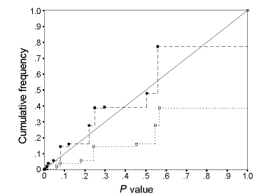
Fig. 1. The cumulative frequency of P values by the K. Pearson chi squared test (-- --) and Fisher-Irwin test by doubling the one-sided value (- - -) for a comparative trial with m = n = 6 and π = 0.5. Points for an ideal test would lie on the diagonal line.
A perfect test will have all points on the diagonal line. From Fig. 1, it is clear that both tests depart from the ideal, for this case of m = n = 6 and π = 0.5. The P values by the Fisher-Irwin test are generally greater than the cumulative frequency by a factor of 2 to 3; for example (referring to the actual values in Table 3), an observed table of (0 6 4 2) has a P value of 6.1%, whereas the cumulative frequency (and so the P value if it were behaving as an ideal test) is 2.1%. This has been a common finding in previous studies (see below), and the Fisher-Irwin test is said to be conservative. The consequence is a loss of power in detecting alternatives to the null hypothesis. The chi squared test has the opposite problem - the P values are generally lower than the cumulative frequency (and so the P value if it were behaving as an ideal test), and so the chi squared test will be misleading in exaggerating the rarity of a table, and so misleading as to the strength of evidence against the null hypothesis (a behaviour sometime termed anticonservative or liberal). The match between the empirical and ideal performance of a test is obviously of most importance at small P values, i.e. at the left of the cumulative frequency chart.
Comparison of actual with nominal Type I error rates and counter-argument of discreteness of P values
A second way to summarise the behaviour of a test for particular values of m, n and π is in terms of the proportion of tables significant under the null hypothesis at a particular level of significance, α, i.e. we compare the actual Type I error with the nominal value α. This is the most common way in which tests have been assessed in previous studies, mostly using nominal significance levels of 5% and 1%, For an ideal test, the actual Type I error will be approximately α, but will be slightly less than α because of the discreteness of the distributions, especially at small sample sizes, as shown in the following example. Consider Table 3 again, when π = 0.5, and assume initially that the ideal test orders the sample space in the same way as the two tests shown. Then we require of the ideal test that the first four tables (0 6 6 0), (0 6 5 1), (0 6 4 2) and (1 5 5 1) will be significant at α = 5%, since these occur with a total frequency of 3.9%, while if the fifth table were also significant, the total frequency rises above 5%. So the ideal test will have a Type I error of 3.9%, i.e. less than the nominal; and so on this measure, even an ideal test will appear conservative. The same argument will hold however the ideal test orders the sample space. This is an important problem because several authors have considered the findings of the conservative behaviour of the Fisher-Irwin test to be either largely or entirely due to this problem of discreteness. For example, Barnard (1979) stated that 'The source of the discrepancy [between the results of the Fisher-Irwin and the Pearson chi squared tests] is much simpler than anything due to loss of information. It is simply the discreteness of the set of possibly P-values'; and Agresti (2001) wrote 'Although some statisticians have philosophical objections to the conditional approach, the root of most objections is their conservatism, because of discreteness. In terms of practical performance the degree of discreteness is the determinant more so than whether one uses conditioning'.
However, referring to Table 3, the actual Type I error for the Fisher-Irwin test at α = 5% is 0.6% at m = n = 6, π = 0.5 (the total frequency of tables with P values less than 5% is 0.6%). If the test was behaving as an ideal test, this value would be 3.9%, as noted above. It is clear that the Fisher-Irwin test is markedly conservative in this example, and that this behaviour is not due to discreteness. A large number of other examples were studied as part of this investigation, and similar findings were made in all cases. As the study size increases, the number of tables increases rapidly, particularly in cross-sectional studies, and this problem of discreteness becomes less important.
Tocher (1950) suggested the Fisher-Irwin test (and other tests) could be modified by drawing a random number after analysis of the data from a study, the number being chosen so that a pre-specified nominal α is matched exactly. This would remove the discrete behaviour, but does not affect the conservative behaviour of the Fisher-Irwin test. More recently, there has been a greater emphasis on giving actual P values from a test rather than deciding between significant and not significant at some arbitrary level.
Criteria for accepting a test as valid
The K. Pearson chi squared test in the above example has Type I error rates that are too high (e.g. 5.8% at a nominal level of 5%). Should we therefore declare the test to be invalid in this situation? One possible policy is that the actual Type I error rate should never be above the nominal level, so that the test never exaggerates the strength of evidence in a study, but most authors have felt that a small excess is allowable. Cochran (1942), in assessing the related problem of the chi squared goodness-of-fit test, suggested that a 20% error be permitted in the estimation of the true probability e.g. an error up to 1% at the 5% level, and up to 0.2% at the 1% level. Subsequently, Cochran (1952) suggested a slightly different criterion that a departure could be 'regarded as unimportant if when the P is 0.05 in the χ2 table, the exact P lies between 0.04 and 0.06, and if when the tabular P is 0.01, the exact P lies between 0.007 and 0.015'. Cochran noted that the criteria are arbitrary, and that others might prefer wider limits, but authors have generally followed one or other of Cochran's suggestions, e.g. Upton (1982).
Using Cochran's original criteria, we would decide that the Fisher-Irwin gives a true Type I error rate that is too low. We might accept the K. Pearson chi squared test as conforming to Cochran's criterion at α = 5%, since the actual value is 5.8%, but this value is considerably in excess of the value of 3.9% for an ideal test with the same sample space ordering. This example shows the drawback in looking at a particular nominal value (α), and an advantage in considering the extent to which Type I errors exceed the nominal value over a range of nominal values. So, for example, we might look at the maximum excess in Type I error over the nominal for nominal values up to 5%. From Table 3, this maximum Type I error excess is the difference of 1.8% in the fourth row between a Type I error of 3.9% (in the cumulative P value frequency column) and the nominal significance level of 2.1% (in the P value column). This would then be judged too large on the criterion that all differences should be less than 20%. The maximum Type I error excess (graphically the maximum height of the cumulative frequency chart above the diagonal) can be looked at another way (graphically the maximum distance of the cumulative frequency chart to the left of the diagonal) i.e. as the maximum extent to which P values exaggerate the rarity of sample tables, which might be termed the P value exaggeration, but this alternative description seems less intuitive. The research shown here presents results on both actual Type I error rates at particular nominal values (as in many previous papers) together with the maximum Type I error excess over a range of nominal values up to a particular value (which is a new technique).
Performance as a function of π and the problem of a zero marginal total
Considering now values of π other than 0.5, in a comparative trial with m = n = 6, we can repeat the relevant calculations of Table 3 and construct charts such as Fig. 1 at a series of values of π. We can then summarise these charts by a plot of the actual Type I error rate for each test at a particular nominal value α against π. For example, Fig. 2 (a) shows the Type I error rate at α = 5% for the example of a comparative trial with m = n = 6.
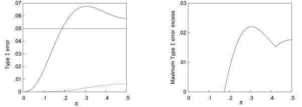
Fig. 2. (a) Type I error rate at a nominal significance level of 5% and (b) maximum Type I error excess for nominal values up to 5% as a function of the population proportion (π) for a comparative trial with m = n = 6, analysed by the K. Pearson chi squared test (---) and Fisher-Irwin test by doubling the one-sided value (- - -).
This method has been used in several previous studies (e.g. Upton, 1982; Storer and Kim, 1990). As noted for π = 0.5, this may not necessarily demonstrate the extent to which Type I errors exceed the nominal, and a more informative plot may be the maximum Type I error excess against π. Fig. 2 (b) shows such a plot for nominal significance levels up to 5% for the same example of a comparative trial with m = n = 6.
Fig. 2 illustrates a number of important points. Firstly, for both tests, the Type I error rate is shown as falling to zero at π = 0. This feature is dependent on how we view the table in the bottom row of Table 3, i.e. (0 6 0 6). Here, one of the marginal totals of the table is zero. So, for example, in a comparison of two treatments, we might find that a particular side-effect that we were recording did not occur at all in either group. In such a case, no statistical test is valid; and generally we would not even consider performing one. The frequency of such a table is negligible when values of π are around 0.5, but comes to dominate all others at values of π close to zero. We could choose to say that such tables should be excluded from any assessment of the performance of a statistical test, so that frequencies of tables are calculated as a proportion of those samples where the statistical test is valid. Alternatively, we might include the table as a valid outcome, and take the P value to be indeterminate and not significant. This is an important distinction in a study of small sample limitations such as this, as the policy chosen has a large bearing on the charts etc generated. Berkson (1978a) in a comparative trial with a zero marginal total calculated a one-sided P value of 1 for the Fisher-Irwin test and for the normal test with Yates's adjustment, and of 0.5 for the normal test (his Table 2), but Barnard (1979) pointed out that this last value is misleading. Camilli and Hopkins (1979) presented their results of Type I errors in Monte Carlo simulations in terms of the proportions of all tables, whether or not the column total was zero. Upton (1982) in comparative trials, considered that where the column marginal totals are equal to zero, the null hypothesis should be accepted. This is the policy adopted in this study, on the basis that a scientist carrying out the research is interested in how unusual is the result observed out of the reference set of all the possible outcomes that might have been observed, rather than taking the reference set to be just those that might have been analysed in a particular way. If the scientist finds, for example, no cases at all of a particular side-effect in either treatment group, this is clear evidence against there being a large difference between the rates of that side-effect for the two groups; it is not just an inconclusive result.
A second feature is that the plot of Type I error (Fig. 2a) shows the maximum for the K. Pearson chi squared test to be not at π = 0.5, but at around 0.3, and here the maximum value is well above 6%, and so the test fails even Cochran's original criterion.
Thirdly, the chart for maximum Type I error excess (Fig. 2b) shows a corresponding peak for the K. Pearson chi squared test at π of around 0.3, and shows the plot to be bimodal in the range up to π = 0.5.
Fourthly, there is a region when π is less than about 0.2 where the K. Pearson chi squared test appears to be valid on even the strictest criteria that the actual Type I error must be less than the nominal, and every P value should be no greater than the cumulative frequency (at this value of α of 5%).
Fifthly, the Fisher-Irwin test by doubling the one-sided value has a Type I error far below the nominal at all values of π, and never has a Type I error excess.
Summary figures
It is not easy to summarise the performance of the K. Pearson chi squared test in the above example at α = 5%. There are some values of π where we might judge the test to be valid, and others where we would judge it to be invalid. In some previous studies, the authors have calculated average Type I errors across a range of values of π at intervals of 0.1, for example Upton (1982) and Hirji et al. (1991). Such an average will of course depend on what range we choose, and whether we put the same weight on each value in the chosen range. It is hard to be confident that any such average will predict the general behaviour of the test in practice in any particular field of research, as we do not generally know what values of π will apply, and we cannot rule out the possibility that a particular field of research will carry out a large proportion of its research in just those values of π that make the test most misleading. It therefore seems preferable to take the maximum Type I error across all values of π as a better summary figure than the average, as has been done in a number of previous studies. Some of these have carried out calculations at values of π at a regular interval such as 0.1 or 0.01 (e.g. Schouten et al., 1980; Haber, 1986), and then simply taken the highest Type I error found; whereas Upton (1982) describes finding the maximum Type I error 'by a simple iterative hunt using the computer'.
The actual Type I error is a sum of polynomials in π and so is a smooth function of π, but it may be multimodal (as has been found for some combinations of m and n) and the peaks may be narrow. So there will be some doubt about whether the maximum value found over a finite number of cases is the true maximum. This uncertainty can be overcome by finding an upper bound that can be shown to be greater than the Type I error for any value of π, and that is only slightly larger than an actual value by some pre-specified difference; this method was used by Suissa and Shuster (1985) and was used in the research discussed here (see Methods page). For the same reason as given before, the maximum Type I error should be supplemented as a summary figure by the maximum Type I error excess across all values of π for nominal levels up to a specified value. Since the minimum actual Type I error is zero for all tests at π = 0, the minimum Type I error cannot be used as a summary measure. Once Type I error rates have been calculated (either the value at a particular value of π or the maximum value across all values of π), these can be plotted against total sample size (as in Storer and Kim, 1990; Hwang and Yang, 2001).
For cross-sectional studies, it is more difficult to investigate actual Type I error rates because we must consider the variation with the two population parameters π1 and π2, and if we want to find maximum values, these must be found across all values of each. Prior to this study, there have been few investigations of the behaviour of tests in cross-sectional studies.
Other empirical methods
Previous studies have included a wide range of other methods of summarising the performance of tests. As computing power has increased, more complex methods of summarising performance have become possible. For example, Upton (1982) looked at the size of the rejection region in terms of the number of sample tables rejected by each of 17 tests in a comparative trial for 12 different combinations of m, n, and α; and Hirji et al. (1991) gave selected percentiles for the distribution of Type I errors for 3125 configurations of m, n and π.
Comparison of tests by Type I error: findings
The first published study was by E. Pearson (1947), who compared versions of the chi squared test with and without Yates's continuity adjustment. Pearson compared actual with nominal one-sided Type I error rates in a comparative trial for two pairs of values of m and n, at two nominal significance levels (5% and 1%), at up to 11 values of π. He concluded that the inclusion of Yates's adjustment 'gives such an overestimate of the true chances of falling beyond a contour as to be almost valueless', whereas using the version without Yates's adjustment gave Type I error rates considerably nearer to the nominal value. He noted that the actual level sometimes exceeded the nominal values but never by very much, and went on to recommend this unadjusted version for analysis of comparative trials in general (except at very small marginal totals), and tentatively came to the same conclusion for cross-sectional studies on theoretical grounds, but noted that more investigation was needed. The unadjusted version of the chi squared test that E. Pearson studied and recommended was in fact the 'N - 1' version, but subsequent authors often seem to have overlooked this.
Since E. Pearson's paper, other similar studies have been carried out and these have progressively become more comprehensive and sophisticated, reflecting the development of computer technology. For example, whereas E. Pearson studied two tests at two significance levels at two combinations of m and n with values of π at an interval of 0.1, Hirji et al. (1991) studied seven two-sided tests at four significance levels, at 625 combinations of m and n, with values of π at an interval of 0.1. Other studies of comparative trials have confirmed the lower than nominal Type I error rates of Yates's chi squared test (Grizzle, 1967, via a Monte Carlo method; Kurtz, 1968; Garside and Mack, 1976; Berkson, 1978a; Camilli and Hopkins, 1978; Upton, 1982; D'Agostino et al., 1988; Richardson, 1990; Hirji et al., 1991), and of the Fisher-Irwin test (Berkson, 1978a; Garside and Mack, 1976; Upton, 1982; Overall et al., 1987; D'Agostino et al., 1988; Hirji et al., 1991); and confirmed that these two tests give very similar P values (Berkson, 1978a; Garside and Mack, 1976; Upton, 1982), as was Yates's intention. Both tests have often been found to give actual Type I error rates less than half of the nominal level across a range of sample sizes and values of π, but especially with small to moderate sample sizes. Although it has been stated frequently that the various tests become equivalent for 'large' N, even at m = n = 100 (and π = 0.5) Berkson (1978a) found appreciable differences between the tests.
K. Pearson's ('N') version of the chi squared test has been confirmed as giving Type I error rates closer to the nominal than Yates's chi squared test and the Fisher-Irwin test (Grizzle, 1967; Roscoe and Byars, 1971; Garside and Mack, 1976; Berkson, 1978a; Camilli and Hopkins, 1978 and 1979; Upton, 1982; D'Agostino et al., 1988). However, Garside and Mack (1976) found that the unadjusted chi squared test could sometimes give Type I errors appreciably larger than the nominal value, especially with values of π away from 0.5, and when m and n are unequal, and this has been confirmed by subsequent studies (Camilli and Hopkins, 1979; Upton, 1982; D'Agostino et al., 1988; Storer and Kim, 1990).
The 'N - 1' chi squared test was re-examined by Schouten et al. (1980), Upton (1982) and Rhoades and Overall (1982). Like E. Pearson (1947), they found it to give Type I error rates in comparative trials closer to nominal values than Yates's chi squared test and the Fisher-Irwin test. Both the last two papers recommended the 'N - 1' version in preference to the 'N' version, although Upton later retracted his opinion (Upton, 1992), after being 'converted' to a conditional approach (see the discussion page). Haber (1986) studied the maximum Type I error rates for the 'N - 1' chi squared test (in its equivalent normal form) across 99 values of π, for all cases of m and n up to 20, and found the maximum rates in many cases substantially exceeded the nominal significance level (even by factors of more than 2). Overall et al. (1987) and Hirji et al. (1991) confirmed that maximum Type I errors by the 'N - 1' chi squared test can be much higher than nominal values, although to a smaller extent than the 'N' version.
Hirji et al. (1991) were the first to study two-sided versions of the Fisher-Irwin test, and found that the method using Irwin's rule was less conservative than the method doubling the one-sided probability. Dupont (1986) pointed out a problem with the two-sided Fisher-Irwin test in that similar sets of data did not give similar P values when calculated by Irwin's rule. In a comparative trial with the outcome (10 90 20 80), this test gives a P value of 7.3%; whereas if the outcome had been (10 91 20 80) (and we would say that the strength of evidence for a difference in success rate is similar), the P value by the test falls to 5.0%. By contrast, the P value by the two-sided Fisher-Irwin test calculated as twice the one-sided test changes much less, from 7.3% to 6.9%, and the P value by the unadjusted chi squared test changes little from 4.8% to 4.5%. Furthermore, Dupont showed that this is a general feature of other pairs of tables that he analyzed. This problem with the Fisher-Irwin test by Irwin's rule reduces our confidence in the P values that it gives.
Hirji et al. (1991) were the first to study mid-P versions of the Fisher-Irwin test in comparative trials. They found that the mid-P method doubling the one-sided probability performs better than standard versions of the Fisher-Irwin test, and the mid-P method by Irwin's rule performs better still in having actual Type I levels closest to nominal levels, although the median level over the range of cases studied was still below nominal levels. Because of the absence of high actual levels, these authors recommended use of the mid-P method by Irwin's rule in preference to the 'N - 1' chi squared test. Hwang and Yang (2001) also judged the mid-P method by Irwin's rule to perform quite reasonably.
Cross-sectional studies have been investigated by fewer authors, but Grizzle (1967), Bradley and Cutcomb (1977), and Camilli and Hopkins (1978 and 1979) using Monte Carlo methods came to conclusions similar to those for comparative trials i.e. that Type I error rates for Yates's chi squared test are considerably below nominal values; and that the unadjusted chi squared test has Type I error rates generally closer to the nominal rate, but sometimes exceeding it especially at low values of π1 and π2. Richardson (1990) carried out both probability calculations and Monte Carlo simulations for two sample sizes and nine combinations of row and column probabilities, and came to similar conclusions; and furthermore repeated the findings seen in comparative trials that the 'N - 1' chi squared test gave Type I errors closer to nominal values than the 'N' version. It is not surprising that the conclusions for cross-sectional studies mirror those for comparative trials as the probabilities for the possible tables in the sample space in a cross-sectional study are the weighted means of those in comparative trials with the same total sample size, with weightings according to the probability of any (m, n) pairing, which is governed by π1.
Martin Andres and Herranz Tejedor (2000) and Martin Andres et al. (2002) studied the performance of various tests when the sample tables were grouped according to the minimum expected cell number. However, the standards by which they assessed validity were the P value by the Fisher-Irwin test in the former study, and the P value by Barnard's test (1947a) in the latter (this ensures that the P value is never above the nominal), and so these are not directly relevant to the questions addressed in the research discussed here. Larntz (1978) looked at the related problem of how well the K. Pearson chi squared test performs in testing multinomial goodness of fit in small samples, where the number of cells is 2, 3, 5 or 10. For a number of different combinations of probabilities, and for sample sizes from 10 to 100, Larntz found that the Type I error is generally close to the nominal value when cell expected numbers are on average greater than 1.0. Camilli and Hopkins (1978) made similar observations in 2 x 2 tables. However, these studies are of average cell frequencies expected from the population parameters that were set. Prior to this research, there seem to have been no studies of the consequences of restricting tests to sample tables where the smallest expected cell number exceeds a particular level.
Power and ordering of the sample space
As Storer and Kim (1990) pointed out, the finding of one test being conservative compared to another would be of little interest unless it translates into a difference in power. Table 4 illustrates the relation in the case of a comparative trial with m = n = 6, analysed by the 'N - 1' chi squared and the Fisher-Irwin test by doubling the one-sided value. It shows the frequencies of the 16 different sample tables under one particular alternative hypothesis, namely a difference in population proportion of 0.2 in one group against 0.6 in the other, and so allows a calculation of the power of the 'N - 1' chi squared and the Fisher-Irwin tests, via summation of the frequencies of those tables significant at 5% by the two tests.
Table 4. The power by the 'N - 1' chi squared test and the Fisher-Irwin test to detect a difference between two population proportions of 0.2 versus 0.6 in a comparative trial with group sizes of six (m = n = 6) at a two-sided significance level of 5%.
| --------------------------------------------------------------------------------------------------- | |||
| Sample table | Frequency | P value (%) where significant | P value (%) where significant |
| (a b c d) | (%) | by the 'N - 1' chi squared test | by the Fisher-Irwin test* |
| --------------------------------------------------------------------------------------------------- | |||
| 0 6 6 0 | 1.2 | 0.09 | 0.2 |
| 0 6 5 1 | 6.7 | 0.5 | 1.5 |
| 0 6 4 2 | 9.3 | 1.9 | - |
| 1 5 5 1 | 7.3 | 2.7 | - |
| 0 6 3 3 | 7.7 | - | - |
| 1 5 4 2 | 16.9 | - | - |
| 0 6 2 4 | 3.8 | - | - |
| 1 5 3 3 | 12.7 | - | - |
| 2 4 4 2 | 7.9 | - | - |
| 1 5 0 6 | 1.1 | - | - |
| 1 5 2 4 | 6.7 | - | - |
| 2 4 3 3 | 10.9 | - | - |
| 3 3 3 3 | 2.3 | - | - |
| 2 4 2 4 | 3.9 | - | - |
| 1 5 1 5 | 1.5 | - | - |
| 0 6 0 6 | 0.1 | not applicable | not applicable |
| Total significant (i.e. power) by the 'N - 1' chi squared test: 24.5% | |||
| Total significant (i.e. power) by the Fisher-Irwin test: 7.9% | |||
| --------------------------------------------------------------------------------------------------- | |||
| *Calculated as double the one-sided P value | |||
The top two sample tables, (0 6 6 0) and (0 6 5 1), are significant at 5% by the Fisher-Irwin test, and occur with a total frequency of 7.9% - so the power of the Fisher-Irwin test to detect a difference in proportion of 0.2 versus 0.6 is just 7.9%. When analysis is done by the 'N - 1' chi squared test, the significant sample tables are now the top four in Table 4, which occur at a total frequency of 24.5% i.e. the power in this situation is 24.5%. The increase in power compared to the Fisher-Irwin test is due to the inclusion of the extra two sample tables in the set of significant tables. This same argument will apply whatever difference in population proportions we are trying to detect (i.e. whatever the alternative hypothesis). Since there are some sample tables significant by the 'N - 1' chi squared test that are not significant by the Fisher-Irwin test, but none the other way around, and since these sample tables will always occur at some non-zero frequency, the power by the 'N - 1' chi squared test will always exceed that by the Fisher-Irwin test in a comparative trial with group sizes of six. This illustrates the principle (Upton, 1982) that if the rejection region for one test is a subset of that for a second test, then the power of the second test will be greater than that of the first for all alternative hypotheses. If some sample tables are significant by the first test but not by the second, while other sample tables are significant by the second test but not by the first, then the question of which test is the more powerful will be settled by the relative frequencies of these two groups of sample tables, which will depend on the alternative hypothesis, and no simple general statement on the relative power will be possible.
Calculations (Berkson, 1978a; Storer and Kim, 1990) and Monte Carlo simulations (Richardson, 1990) in a limited number of particular alternative hypotheses have shown that both the Fisher-Irwin test and Yates's chi squared test are less powerful than the K. Pearson chi squared test in those situations studied, but these investigations of particular situations are limited by the large number of different null and alternative hypotheses possible. Prior to the research discussed on these pages, there seem to have been no systematic comparisons of the sets of sample tables significant by the tests under scrutiny.
Summary of previous research
It is desireable to have a test of 2 x 2 tables that has Type I error rates as close as possible to the nominal significance level over a wide range of population proportions, and over a range of sample sizes to as low as possible. If Type I error rates are too high, the test is invalid because it is misleading. If Type I error rates are too low, the test is valid, but it is a poor test because it is not as good at picking up real differences as it could be, i.e. it has low power.
The K. Pearson and 'N - 1' chi squared tests cannot be used at low sample sizes without restriction because they have Type I error rates considerably above the nominal, across certain ranges of the unknown population proportion(s). In these circumstances, (and also, some would say, for theoretical reasons detailed in the discussion sections), the Yates chi squared test and the Fisher-Irwin test are generally substituted, resulting in low Type I error rates, and inevitable loss of power. Restrictions on when the K. Pearson chi squared test can be used date back over 50 years to Cochran and earlier. Cochran noted that the restrictions were arbitrary and provisional, giving rise to a clear need for further research on the performance of variants of the chi squared test under various restrictions.
The research presented on these pages aimed to address this need for further research. The approach taken was to take advantage of increases in computing power to develop software that allowed a large number of summary charts to be generated and viewed in a short period of time, and consequently enabled a comprehensive understanding of the problem. The software is made available in order to hasten the achievement of a consensus on new recommendations.
Back to top